MATLAB and Python
Installing Python for Matlab (Windows)
Versions of Python Compatible with MATLAB Products by Release (Note: As of MATLAB R2023a, Python 2.x is no longer supported.)
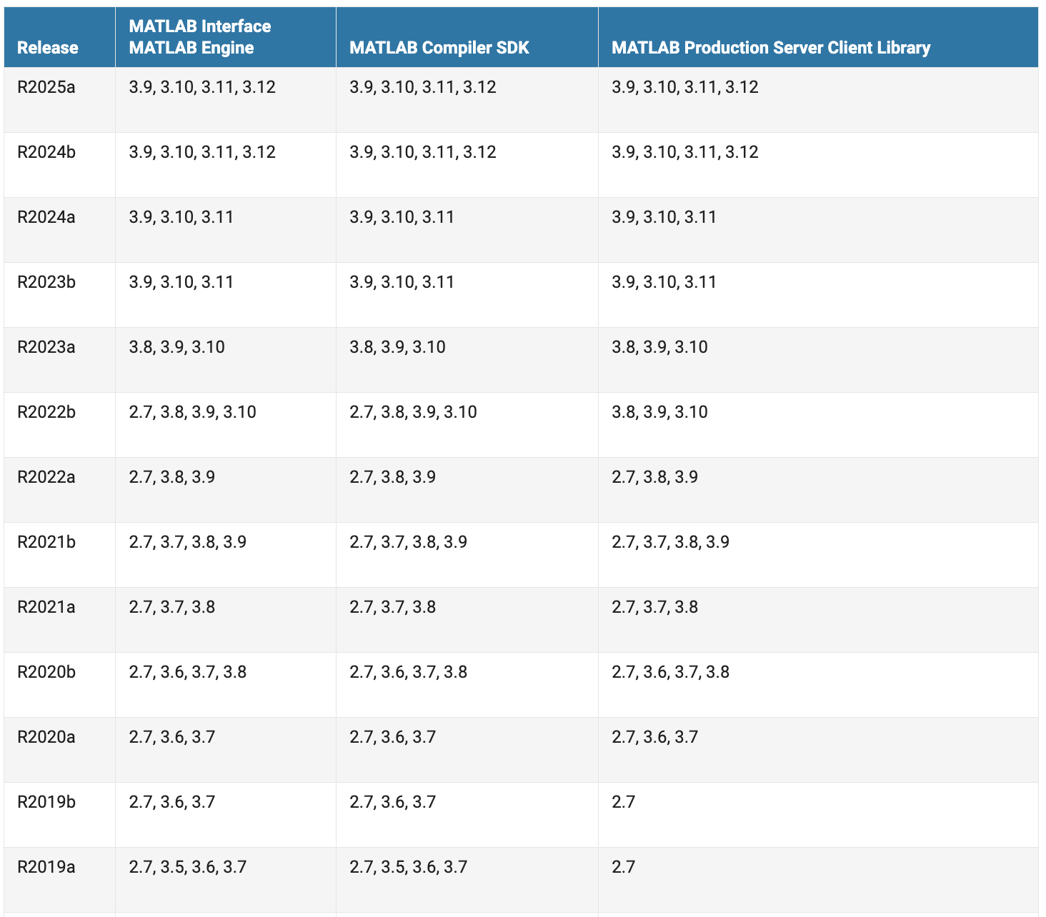
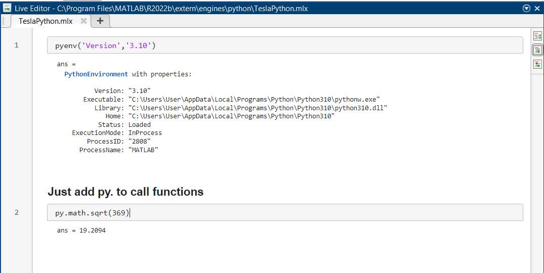
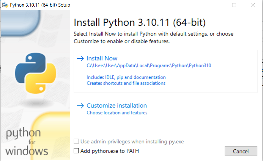
According to the above table, we use MATLAB R2022b so we will install Python 3.10 After that, check that Matlab can recognize the Python installation by typing pyenv in Command Window of Matlab.
Installing Matlab for Python (Windows)
Let’s see how we can set default Python version on Windows. As you can see I have three versions of Python installed.
cmd¶> py -0
-V:3.12 * Python 3.12 (64-bit)
-V:3.11 Python 3.11 (Store)
-V:3.10 Python 3.10 (64-bit)
> python --version
Python 3.11.4
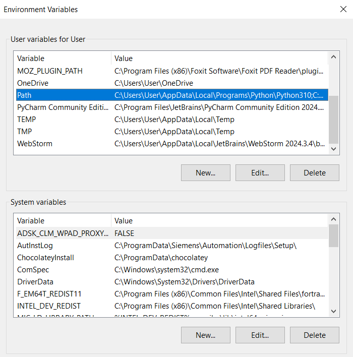
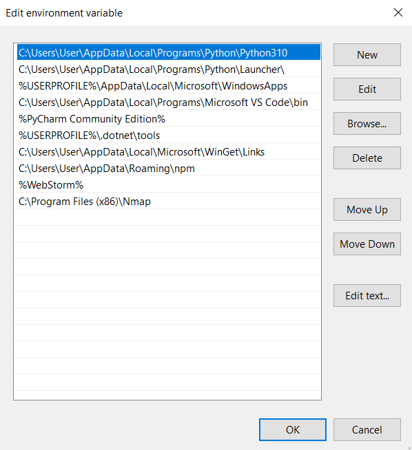
To set up the default Python 3.10, open Edit The System Environment Variables –> click Environment Variables –> double click Path –> click New –> creat C:UserUserAppDataLocalProgramsPythonPython310 like the path as install Python. And then Move it Up on the top. Closing all.
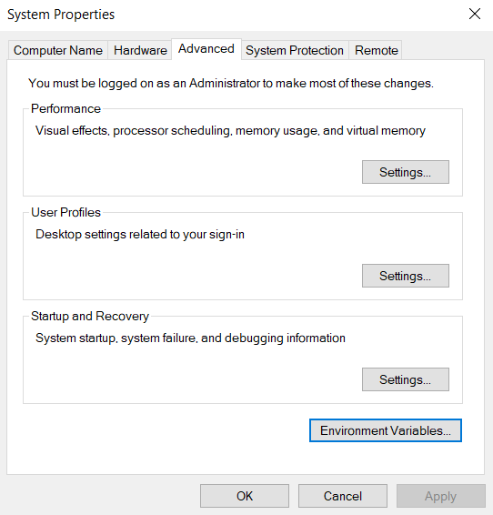
Open cmd again, done
cmd¶> python --version
Python 3.10.11
Checking up MATLAB root in order to install matlabengine
Command Window of MATLAB¶>> matlabroot
ans =
'C:\Program Files\MATLAB\R2022b'
Checking up MATLAB name
Command Window of MATLAB¶>> matlab.engine.shareEngine
>> matlab.engine.engineName
ans =
'MATLAB_2808'
Open cmd of Wnidows and using your MATLAB root
cmd¶> cd C:\Program Files\MATLAB\R2022b\extern\engines\python
> python -m pip install .
Successfully built matlabengineforpython
Installing collected packages: matlabengineoforpython
Successfully installed matlabengineforpython-9.13
Now we could use MATLAB with Python
cmd¶>python
Python 3.10.11
>>> import matlab.engine
>>> m = matlab.engine.connect_matlab('MATLAB_2808')
>>> x = m.sqrt(369)
>>> print(x)
19.2094
Matlab with Python for AI
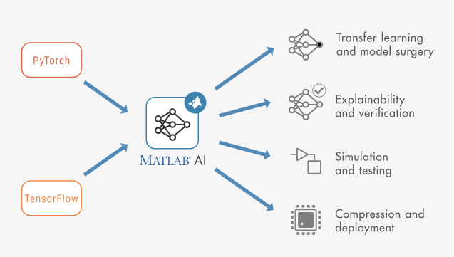
By integrating with PyTorch and TensorFlow, MATLAB enables you to:
Facilitate cross-platform and cross-team collaboration
Test model performance and system integration
Access MATLAB and Simulink tools for engineered system design
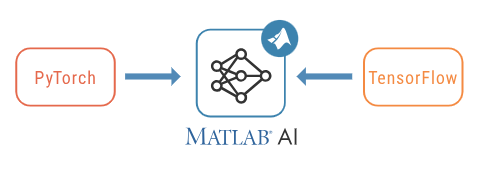
Convert Between MATLAB, PyTorch, and TensorFlow
With Deep Learning Toolbox and MATLAB, you can access pretrained models and design all types of deep neural networks. But, not all AI practitioners work in MATLAB. To facilitate cross-platform and cross-team collaboration when designing AI-enabled systems, Deep Learning Toolbox integrates with PyTorch and TensorFlow.
Why import PyTorch and TensorFlow models into MATLAB
When you convert a PyTorch or TensorFlow model to a MATLAB network, you can use your converted network with all MATLAB AI built-in tools, such as functions and apps, for transfer learning, explainable AI and verification, system-level simulation and testing, network compression, and automatic code generation for target deployment.
Prepare PyTorch and TensorFlow models for import
Before importing PyTorch and TensorFlow models into MATLAB, you must prepare and save the models in the correct format. You can use the code below in Python to prepare your models.
The PyTorch importer expects a traced PyTorch model. After you trace the PyTorch model, save it. For more information on how to trace a PyTorch model, go to Torch documentation: Tracing a function.
X = torch.rand(1,3,224,224)
traced_model = torch.jit.trace(model.forward,X)
traced_model.save("torch_model.pt")
Your TensorFlow model must be saved in the SavedModel format.
model.save("myModelTF")
How to import PyTorch and TensorFlow models
You can import models from PyTorch and TensorFlow into MATLAB, converting them into MATLAB networks with just one line of code.
Use the importNetworkFromPyTorch function and specify PyTorchInputSizes with the correct input size for the specific PyTorch model. This allows the function to create an image input layer for the imported network because PyTorch models do not inherently have input layers. For more information, see Tips on Importing Models from PyTorch and TensorFlow.
To import a network from TensorFlow, use the importNetworkFromTensorFlow function.
Import PyTorch and TensorFlow models interactively
You can import models from PyTorch interactively with the Deep Network Designer app. Then, you can view, edit, and analyze the imported network from the app. You can even export the network directly to Simulink from the app.
How to export models from MATLAB to PyTorch and TensorFlow
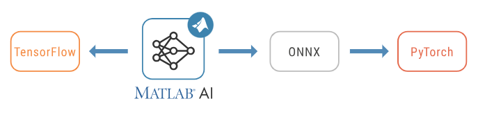
You can export and share your MATLAB networks to TensorFlow and PyTorch. Use exportNetworkToTensorFlow to directly export to TensorFlow and the exportONNXNetwork function to export to PyTorch via ONNX™.
exportNetworkToTensorFlow(net,"myModel")
Matlab and Python with Predictive Maintenance for Motors
Identifying motor fault using Machine Learning for PM(Predictive Maintenance) Detecting amd diagnosing rotor broken bar in a three-phase inductive motor. Ten experiments were performed for each combination of health and loading condition. The following signals were acquired during each experiment:
Voltage of each phase (Va, Vb, Vc)
Current draw of each phase (Ia, Ib, Ic)
Mechanical vibration speeds tangential to the housing (Vib hous) and base (Vib base)
Mechanical vibration speeds axial on the driven side (Vib axial)
Mechanical vibration speeds radial on the driven side (Vib radial_N) and non-driven side (Vib radial_ND)
Extract the compressed data files into the current folder.
unzip(filename)
Extract Ensemble Member Data
Convert the original motor data files into individual ensemble member data files for all combinations of health condition, load torque, and experiment index. The files are saved to a target folder and used by the fileEnsembleDatastore object in the Diagnostic Feature Designer app for data processing and feature extraction.
numExperiments = 10;
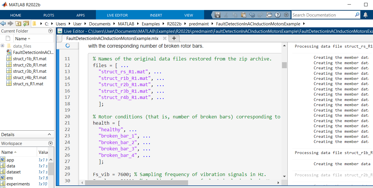
The unzipped files of the original data set are associated with different numbers of broken rotor bars. Create bookkeeping variables to associate the original data files with the corresponding number of broken rotor bars.
% Names of the original data files restored from the zip archive.
files = [ ...
  "struct_rs_R1.mat", ...
  "struct_r1b_R1.mat", ...
  "struct_r2b_R1.mat", ...
  "struct_r3b_R1.mat", ...
  "struct_r4b_R1.mat", ...
  ];

% Rotor conditions (that is, number of broken bars) corresponding to original data files.
health = [
  "healthy", ...
  "broken_bar_1", ...
  "broken_bar_2", ...
  "broken_bar_3", ...
  "broken_bar_4", ...
  ];

Fs_vib = 7600; % Sampling frequency of vibration signals in Hz.
Fs_elec = 50000; % Sampling frequency of electrical signals in Hz.
Create a target folder to store the ensemble member data files that you generate next.
folder = 'data_files';
if ~exist(folder, 'dir')
  mkdir(folder);
end
Construct File Ensemble Datastore
Create a file ensemble datastore for the data stored in the MAT-files, and configure it with functions that interact with the software to read from and write to the datastore.
location = fullfile(pwd, folder);
ens = fileEnsembleDatastore(location,'.mat');
Before you can interact with data in the ensemble, you must create functions that tell the software how to process the data files to read variables into the MATLAB workspace and to write data back to the files. For this example, use the following supplied functions.
readMemberData — Extract requested variables stored in the file. The function returns a table row containing one table variable for each requested variable.
writeMemberData — Take a structure and write its variables to a data file as individual stored variables.
ens.ReadFcn = @readMemberData;
ens.WriteToMemberFcn = @writeMemberData;
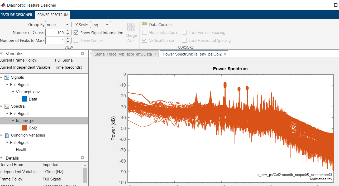
Finally, set properties of the ensemble to identify data variables, condition variables, and the variables selected to read. These variables include ones that are not in the original data set but rather specified and constructed by readMemberData: Vib_acpi_env, the band-pass filtered radial vibration signal, and Ia_env_ps, the band-pass filtered envelope spectrum of the first-phase current signal. Diagnostic Feature Designer can read synthetic signals such as these as well.
ens.DataVariables = [...
  "Va"; "Vb"; "Vc"; "Ia"; "Ib"; "Ic"; ...
  "Vib_acpi"; "Vib_carc"; "Vib_acpe"; "Vib_axial"; "Vib_base"; "Trigger"];
ens.ConditionVariables = ["Health"; "Load"];
ens.SelectedVariables = ["Ia"; "Vib_acpi"; "Health"; "Load"];

% Add synthetic signals and spectra generated directly in the readMemberData
% function.
ens.DataVariables = [ens.DataVariables; "Vib_acpi_env"; "Ia_env_ps"];
ens.SelectedVariables = [ens.SelectedVariables; "Vib_acpi_env"; "Ia_env_ps"];
Examine the ensemble. The functions and the variable names are assigned to the appropriate properties.
ens
Examine a member of the ensemble and confirm that the desired variables are read or generated.
T = read(ens)
From the power spectrum of one of the vibration signals, Vib_acpi, observe that there are frequency components of interest in the [900 1300] Hz region. These components are a primary reason why you use readMemberData to compute the band-pass filtered variables - Vib_acpi_env and Ia_env_ps.
% Power spectrum of vibration signal, Vib_acpi
vib = T.Vib_acpi{1};
pspectrum(vib.Data, Fs_vib);
annotation("textarrow", [0.45 0.38], [0.65 0.54], "String", "Fault frequency region of interest")
The envelope of signals after band-pass filtering them can help reveal demodulated signals containing behavior related to the health of the system.
% Envelop of vibration signal
y = bandpass(vib.Data, [900 1300], Fs_vib);
envelope(y)
axis([0 800 -0.5 0.5])
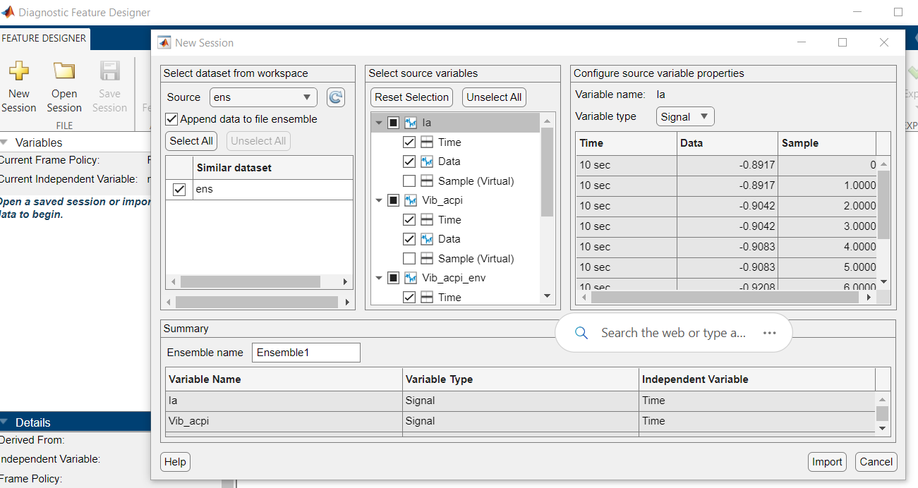
Import Data into Diagnostic Feature Designer App
Open the Diagnostic Feature Designer app using the following command.
app = diagnosticFeatureDesigner;
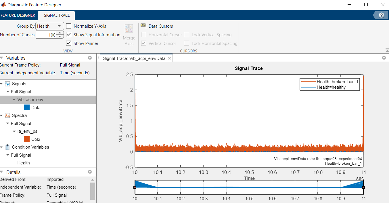
Diagnostic Feature Designer:
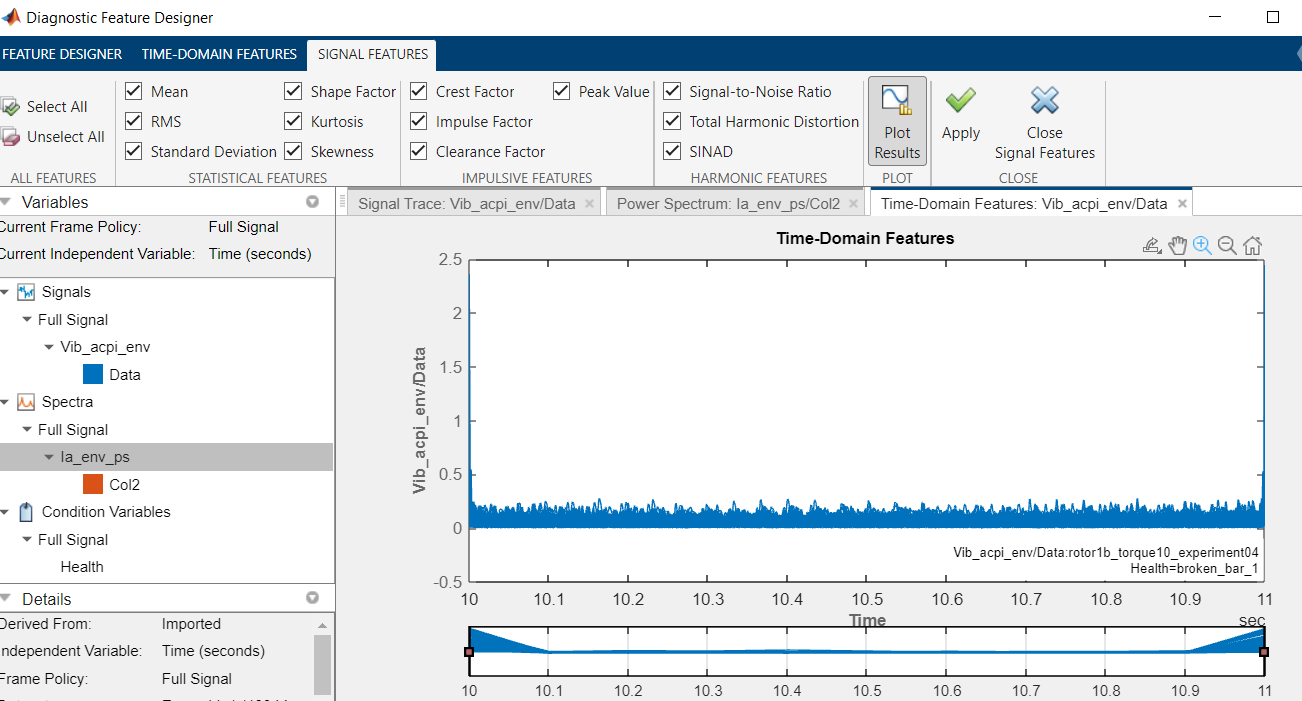
Signal Trace:
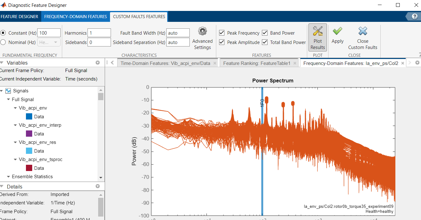
Power Spectrum:
Signal Features:
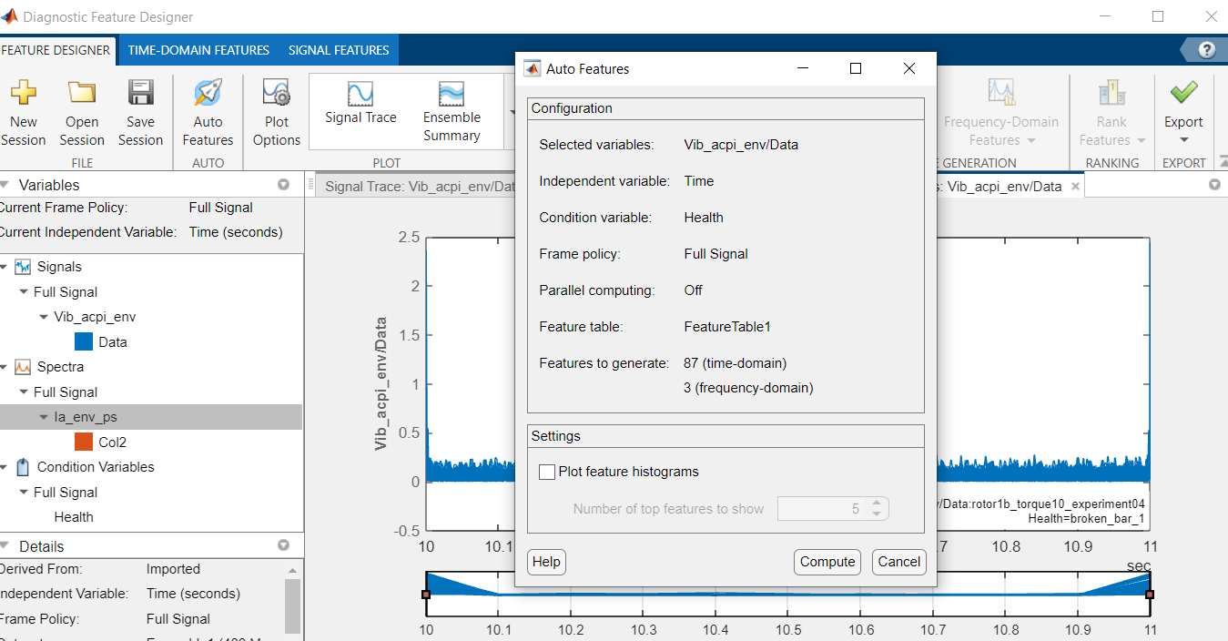
Auto Features:
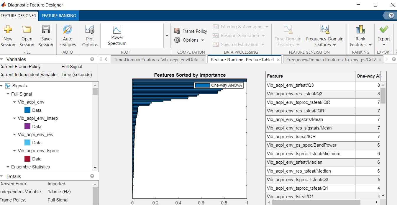
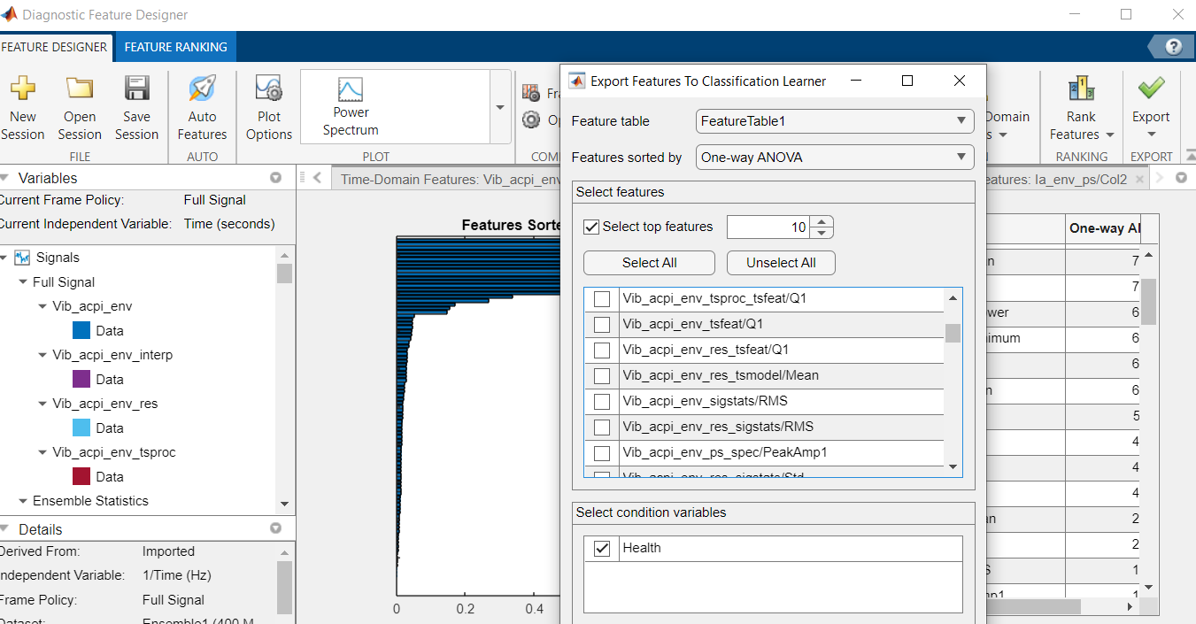
One-way ANOVA test:
Custom Faults Features:
Export Feature To Classification Learner:
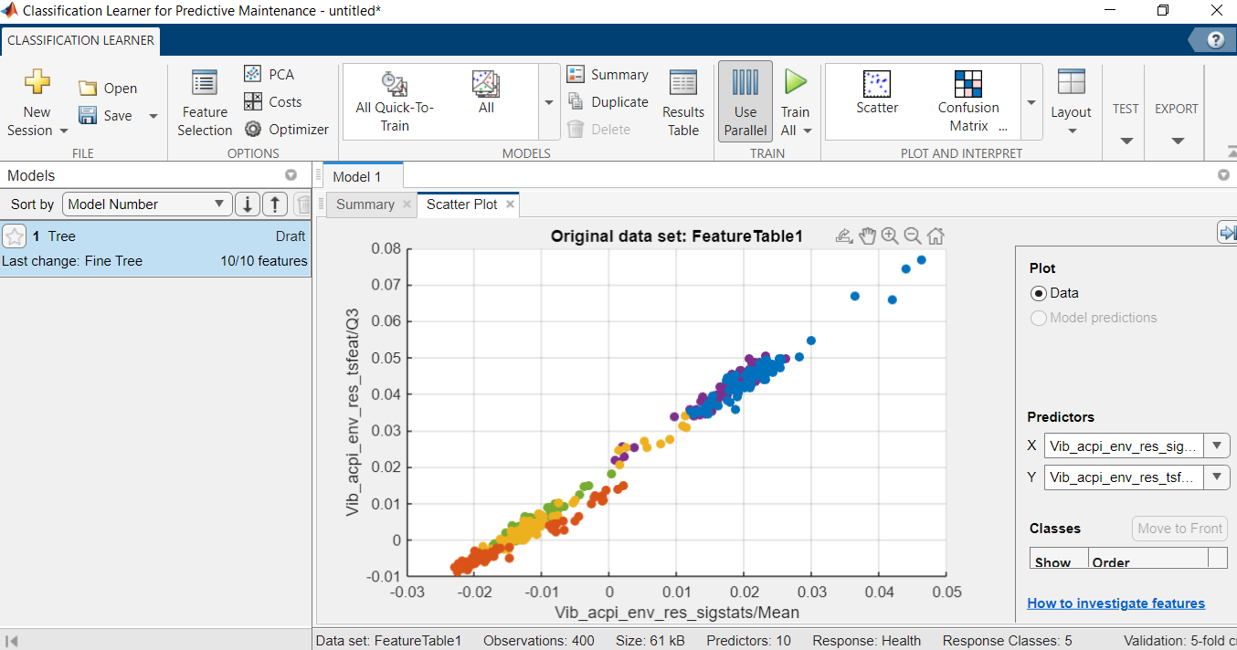
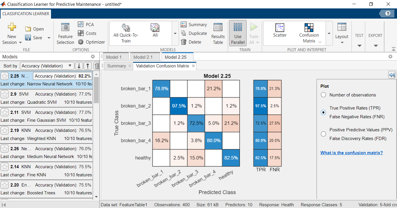
Classification Learner for Predictive Maintenance (PM)
The final results for PM with the accuracy of 97.5% broken bar No.2:
Matlab and Python for ball bearing fault diagnosis
Problem overview
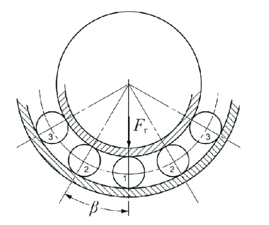
Localized faults in a rolling element bearing may occur in the outer race, the inner race, the cage, or a rolling element. High frequency resonances between the bearing and the response transducer are excited when the rolling elements strike a local fault on the outer or inner race, or a fault on a rolling element strikes the outer or inner race. The problem is how to detect and identify the various types of faults.
Envelope Spectrum Analysis for Bearing Diagnosis
The shaft speed is constant, hence there is no need to perform order tracking as a pre-processing step to remove the effect of shaft speed variations.
dataInner = load(fullfile(matlabroot, 'toolbox', 'predmaint', ...
'predmaintdemos', 'bearingFaultDiagnosis', ...
'train_data', 'InnerRaceFault_vload_1.mat'));
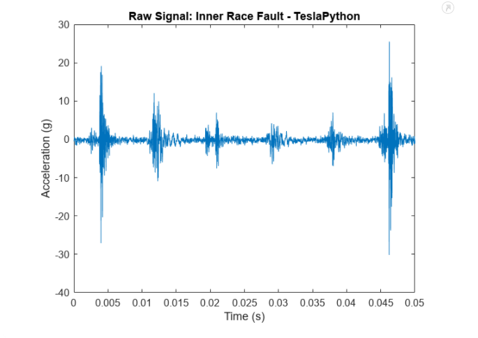
Visualize the raw inner race fault data in the time domain.
xInner = dataInner.bearing.gs;
fsInner = dataInner.bearing.sr;
tInner = (0:length(xInner)-1)/fsInner;
figure
plot(tInner, xInner)
xlabel('Time (s)')
ylabel('Acceleration (g)')
title('Raw Signal: Inner Race Fault - TeslaPython')
xlim([0 0.05])
Now take a closer look at the frequency response at BPFI and its first several harmonics.
figure
[pInner, fpInner] = pspectrum(xInner, fsInner);
pInner = 10*log10(pInner);
plot(fpInner, pInner)
ncomb = 16;
helperPlotCombs(ncomb, dataInner.BPFI)
xlabel('Frequency (Hz)')
ylabel('Power Spectrum (dB)')
title('Raw Signal: Inner Race Fault')
legend('Power Spectrum', 'BPFI Harmonics - TeslaPython')
xlim([0 2000])

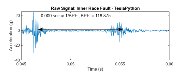
Looking at the time domain data, it is observed that the amplitude of the raw signal is approximately 0.009 sec.
This indicates that the bearing potentially has an inner race fault.
figure
subplot(2, 1, 1)
plot(tInner, xInner)
xlim([0.045 0.060])
title('Raw Signal: Inner Race Fault - TeslaPython')
xlabel('Time (s)')
ylabel('Acceleration (g)')
annotation('doublearrow', [0.22 0.66], [0.8 0.8])
text(0.047, 20, ['0.009 sec \approx 1/BPFI, BPFI = ' num2str(dataInner.BPFI)])
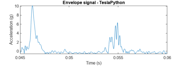
To extract the modulated amplitude, compute the envelope of the raw signal, and visualize it on the bottom subplot.
subplot(2, 1, 2)
[pEnvInner, fEnvInner, xEnvInner, tEnvInner] = envspectrum(xInner, fsInner);
plot(tEnvInner, xEnvInner)
xlim([0.045 0.060])
xlabel('Time (s)')
ylabel('Acceleration (g)')
title('Envelope signal - TeslaPython')
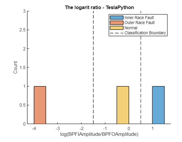
The logarit ratio of the two existing features of BPFI amplitude and BPFO Amplitude that shows a clear separation among the three different bearing conditions.
Last update:
Jul 28, 2025